How to Use Vlookup with a Drop-Down List
Let’s expand your drop-down list using this simple trick in Excel. Teach yourself here how to automatically load the values into the drop-down list using VLOOKUP function.
Table of Contents
Data preparation
The VLOOKUP function in Excel can be used in combination with a drop-down list to return a value based on the selected item in the list. Here’s how you can do it:
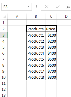
First, prepare the sample table.

Inserting a drop down list
In any cell create, a drop-down list to choose the products from sample the data you’ve just created. Use data validation for that.

Click on the cell right next to the drop-down list.
Vlookup formula to autopopulate a list
Write the formula =VLOOKUP (value you are looking for, table array, column number, false). The formula should include the cell reference of the drop-down list, the data table, and the column number that contains the value you want to return.
If you can’t write that formula, just copy/paste mine: =VLOOKUP(E3;B3:C10;2;0).
Press the Enter key to apply the formula. The result will be the value associated with the selected item in the drop-down list. Your spreadsheet is complete:

Test the drop-down list by selecting different items from the list. The value in the cell with the VLOOKUP formula should change to reflect the selected item.
This is how you can use the VLOOKUP function with a drop-down list in Excel. The VLOOKUP function is a powerful tool that can help you automate data lookup and return values based on the selected item in a drop-down list. Keep in mind that the data table and the drop-down list must be set up correctly for the VLOOKUP function to work as expected.
Using the VLOOKUP Function to Populate a Drop-Down List with Multiple Items
The VLOOKUP function can also be used to populate a drop-down list with multiple items. To do this, you can use the following formula:
=VLOOKUP(lookup_value, table_array, col_index_num, range_lookup)
- lookup_value: The value that you want to look up.
- table_array: The range of cells that contains the data that you want to look up.
- col_index_num: The number of the column that contains the value that you want to return.
- range_lookup: A Boolean value that specifies whether you want an exact match or an approximate match.
For example, the following formula would populate a drop-down list with the names of all of the states in the United States:
=VLOOKUP(“*”, “States”, 2, FALSE)
This formula would look up all of the cells in the States range that start with the value “*”. The value 2 specifies that the column that contains the state names is the second column in the States range. The value FALSE specifies that you want an exact match.
You can use the same formula to populate a drop-down list with any other type of data. Just make sure that the data in the table_array range is sorted in ascending order by the column that contains the value that you want to return.
Here you can download this spreadsheet for free.


Leave a Reply