How to Do Fourier Analysis in Excel
Excel contains a data analysis add-in that allows to to perform a Fourier analysis of a series of numbers. Follow these detailed steps below to execute Fourier analysis in Excel successfully.
Installing Analysis Toolpak
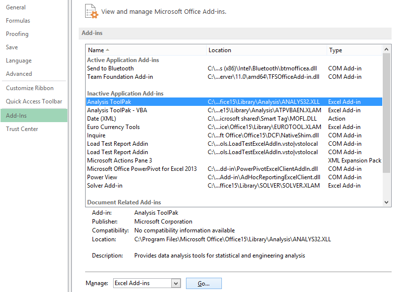
Install the Excel Analysis ToolPak. Launch Excel and click on the “File”. Select “Options” and then click on “Add-Ins”. Click the drop-down menu next to “Manage” at the bottom of the window and then click “Go”. Click the check-box next to “Analysis ToolPak” and then click “OK”.

Enter the number of data points for your Fourier series analysis.
IMPORTANT: In the Fourier series the data must be in the multiples of 2 and cannot exceed 4096.
Evaluating Fourier series
Click on the “Data” tab then click “Data Analysis” in the “Analysis” group. Choose “Fourier Analysis” and click “OK”. A dialog box will appear with options for the analysis.


Click in the “Input Range” box in the dialog that appears. Click and drag on the spreadsheet to highlight the data you want to analyze.

Click in the “Output Range” box and then click and drag on the spreadsheet where you want the analysis to appear. Click OK.

Click and drag on the spreadsheet to select the column or row where your Fourier analysis appeared. Click on the “Insert” tab, click “Scatter” and choose “Scatter with Smooth Lines”. The Fourier series will be plotted as a curve on your graph.


Oscar
hi!,I love yⲟur writing so so much!