How To Create An Attendance Sheet In Excel
Are you looking for an easy way to keep track of attendance for your classes, events or meetings? If so, Excel is a great tool to use. In this Excel tutorial, we’ll show you how to create an attendance sheet in Excel. We’ll walk you through the process step-by-step, so you can get started tracking attendance right away. Whether you’re a teacher, student, or business professional, this tutorial will come in handy.
There are many reasons why you might need to create an attendance sheet. For example, if you’re a teacher, you may need to track student attendance to provide accurate grades. If you’re a business professional, you may need to keep track of employee attendance to meet deadlines or budget restrictions. No matter what your needs are, an attendance sheet can come in handy. Let’s get started!
Table of Contents
How to create an attendance sheet
When creating an attendance sheet in Excel, the first step is to decide what information you want to track. For example, you may want to track the name of each attendee, the date and time of the meeting, or the location of the meeting. Once you know what information you want to track, you can start building your spreadsheet.
The first thing you need to do is open a new Excel spreadsheet. Then, you’ll need to enter in some basic information and decide the layout.
We will use the scenario of Mrs. Green, a teacher looking to track attendance for her English class.
Open the worksheet How To Create An Attendance Sheet In Excel.xlsx, the students’ names are already listed.
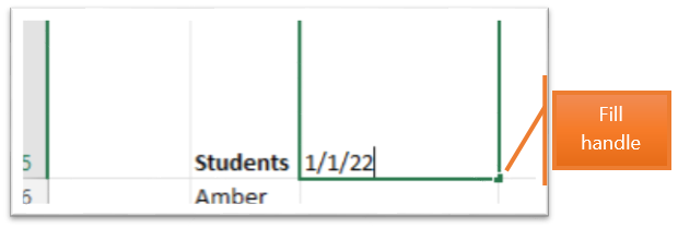
In C5, type 1/1/22, place your cursor over the fill handle, the box in the bottom right of the cell, your cursor turns into a + sign.

Left-click the fill handle, drag it to the right. Excel starts to fill in the dates, drag the handle to 10th January.
Select cells C5:L5 dates, on the Home tab, Alignment group, click Orientation, select Rotate Text Up.

Select columns C – L, drag the left border to reduce the width of the columns to the text.

Make the following entries:
- M5 – Present
- N5 – Absent
- O5 – Attendance %
Use the Orientation tool again, select Rotate Text Up to adjust these three labels.

To capture a count of the students that are Present or Absent we will use the COUNTIF function. We will use the letters P for Present and A for Absent and must place those letters in speech marks for the formula to recognize the text.
In cells C6 through L6 enter the letter P for present.
In M6 enter =COUNTIF(C6:L6,”P”). You should get a count of 10
In N6 enter =COUNTIF(C6:L6,”A”). You should get a count of 0

Let’s change the last three classes for Amber to absent, A. The sheet now shows that Amber was present for 7 sessions and absent for 3.

The COUNTIF function is not case sensitive; you can enter either upper case or lower case A.
Mrs. Green wants to track the attendance rate for each student. To do that she creates a formula that calculates the number of days Amber is present as a percentage of the total number of days in the period (10 days).
To count the range of cells, we’ll use the COUNTA function; this function count cells that are not empty and so is useful when cells contain text. The COUNT function is used to count cells with numbers.
- In O6 enter =M6/COUNTA(C6:L6); the result is 7.
- Stay in O6, on the Home toolbar, Number group, click the % sign.
- Amber has an attendance rate of 70%

Formatting the attendance sheet
Now that we have created a formula to automate the attendance sheet we can copy the formulas to the remaining rows, to the rest of the students, and format the sheet.
- Select C6 through O6, double-click the fill handle. Excel copies the entries and formulas to the remaining students.
- Select the whole table B5 through O19.
- On the Home tab click Format as Table, choose one of the formats.
- The Create Table dialog box opens, click OK. Excel applies the format you selected.

The labels are difficult to read, we can adjust the alignment to correct that.

- Select B5 through O5.
- On the toolbar in the Alignment group, select the Middle Align and Center buttons to center the labels.
- Adjust the height of the row if necessary.


Select and delete all the entries C6 through L19.
Notice the attendance rate entries have an error message, this is because Excel is dividing by zero as the data cells are empty. We can adjust the formula in the attendance column to prevent error messages from appearing when the rows are empty.

Click in O6 enter =IFERROR(M6/COUNTA(C6:L6),” “), the errors disappear.
Using the IFERROR function tells Excel what to display if an error message is triggered in this cell. In this case, the empty speech marks will display an empty cell. When you make entries in the data cell, the formula will still perform as expected.
Make the entries below:
- C6 – P
- D6 – A
- The Attendance rate shows 5
- Select column O, apply the % format.
In the screenshot below, the formula has been applied to all the students. Note Brittney has no entries; her attendance rate is blank. Amber’s attendance rate is calculated on the two entries in her record.


Enter data in all the data cells for the students, be sure to include a mix of absent and present entries.
If Mrs. Green wanted to also have an attendance by class figure, she could create a formula to calculate those present as a percentage of the total amount of students. In writing the formula, Mrs. Green also needs to prevent the empty cells from causing error messages.
- In C20 type =IFERROR(COUNTIF(C6:C19,”P”)/COUNTA(C6:C19),0). Note in this formula, the IFERROR function displays 0 (zero) if an error occurs
- In C20 click the % format
- In the 1/1/22 class, note Amber and Brittany as absent, the remaining students as present.
- You should have an 86% attendance rate for this class.
- Using the fill handle to fill the contents of C20 to L20.

Once you have all this information in your spreadsheet, your attendance sheet is ready to use. Simply enter in the names and ID numbers of the people who will be tracked, and then enter in their attendance status for each day. Excel will automatically calculate the total attendance for you.
How to use formulas and conditional formatting in Excel to track employee attendance
When tracking employee attendance, you can use formulas and conditional formatting to automate the process.
For example, you can use a formula to calculate the number of days each employee has been absent. Then, you can use conditional formatting to highlight employees who have missed more than a certain number of days. This can be a helpful way to quickly see which employees need improvement in attendance.
In our example from above, Mrs. Green wants to quickly view absences.
Select C6:L19.
Click Conditional Formatting.
Click Highlight cell Rules, then Equal To.

The Equal To dialog opens.
In Format cells that are equal to type A.
In the dropdown field choose which format you wish to apply. Note as you select each format option Excel displays a preview of your choice in the background.
Click OK.
Excel applies the conditional format, change any of the absent entries to present, the formatting returns to normal.

Saving your attendance sheet as a template
When creating any type of spreadsheet, it’s important to make sure the data is easy to read and understand. For attendance sheets, this means including headings and labels for each column of data. You may also want to use colors or bold text to highlight important information.
Additionally, it’s a good idea to save your attendance sheet as a template so you can reuse it in the future.
Creating a template from a workbook
Open the document you wish to use as the template.
Save your original document.
Remove any information that you’ll need to change when reusing the spreadsheet – name, dates, etc. Delete the student names, attendance entries, dates and the title in A1.
Click File, Save As.
Enter a name for your template.
Select Excel Template (*.xltx).
Click Save.

Excel creates and opens the template and closes your original document.

Click File, Close to close the template.
Accessing your custom templates – pinned document
To open a template you have created.
- Click File, find your template in the Recent list, click the pin icon.
- When you wish to open the template, click File, click Pinned, find and click your template.

Saving Templates To A Default Drive
We can also tell Excel where to save our templates
- On the menu, click File, Options
- Click the Save tab
- Copy the path in the Default local file location
- Paste the path in the Default personal templates location add \Custom Office Templates to the end
- Click OK
- You may receive an error, if so you’ll need to add the following directory to the systems that are having this issue:
- C:\Users\userid\AppData\Roaming\Microsoft\Excel\URL\
- Once you have created the new location all your templates will be in the Custom Office Templates subfolder in your Documents.

Accessing a custom template – Custom templates folder
- File, New.
- Click the Personal tab.
- Right-click the relevant template, choose Create.

How to password protect an Excel attendance sheet
Creating an attendance sheet can take quite a bit of work – deciding on the information you want to capture, formatting the layout and creating the relevant formulas. Saving attendance sheets as a template prevents you having to recreate the sheets for similar projects.
Another issue to keep in mind when creating attendance sheets is protecting the formulas within your sheet, specifically if others will be making entries for you.
Follow the steps below to protect the formula cells:
Select B6:L19, hold down the CTRL key, select C20:L20
Right-click on the selection, choose Format cells.
Click the Protection tab, deselect Locked, click OK.

On the toolbar, click the Review tab, Protect group, Protect Sheet
Enter the password Sheet,
Under Allow users of this worksheet to: click Select unlocked cells, deselect any other options here.
Click OK.
Reenter the password if necessary.
Try to type in one of the formula fields, M6, you should not be able to select it.
Enter A in C6, your entry is accepted, and updates the result in M6.
The formula is protected but entries in the other cells is permitted.

Removing the lock
How to remove the lock so you can edit the formulas
- On the Review tab, Protect group, click Unprotect Sheet, type in the password, OK
- You can now make changes to any of the cells you have locked.
How to use built-in Excel templates
If you want to create an attendance sheet quickly and easily, you can use an Excel template. Excel templates are pre-made spreadsheets that have all the formatting and formulas in place. This means all you need to do is enter your data and you’re good to go!
There are several different Excel templates available online, or you can create your own. To create a custom Excel template, open a new spreadsheet and save it as a template. This will make it available for future use. You can also password protect your template so that other users can’t change the contents.
- Click File, New.
- In the search for online templates search field type ‘attendance’, a list of possibilities Appear.
- Choose your preference and double-click to open it.
- The first tab of the workbook has information on how to use the template.

Excel is a powerful tool for tracking all sorts of data. With the right formulas and conditional formatting, you can use it to keep track of employee attendance or absences. Hopefully, this Excel tutorial article has shown you how easy it is to create an attendance sheet in Excel and how to use its features to your advantage.


Leave a Reply