How To Use XLOOKUP Function In Excel
The XLOOKUP function is a powerful tool that can be used in Excel to lookup values in a table. It can be used to return information from a single row or column in a table.
The benefits of using XLOOKUP include the ability to quickly and easily find information, as well as the ability to perform complex lookups. In this Excel tutorial lesson, we will discuss how to use the XLOOKUP function in Excel and provide some examples of how it can be used in the real world.
XLOOKUP Syntax
The syntax for XLOOKUP is:
=XLOOKUP(lookup_value, lookup_array, return_array, [if_not_found], [match_mode], [search_mode])
- Lookup value – The item you want to lookup, the data you want to search for.
- Lookup array – The range of cells that contains the data you want to lookup. This is called the lookup range.
- Return array – The range that contains the value you want to return.
Now that we know what each argument represents, let’s take a look at how to use the XLOOKUP function in a real-world example. Open How To Use The XLOOKUP Function In Excel.xlsx.
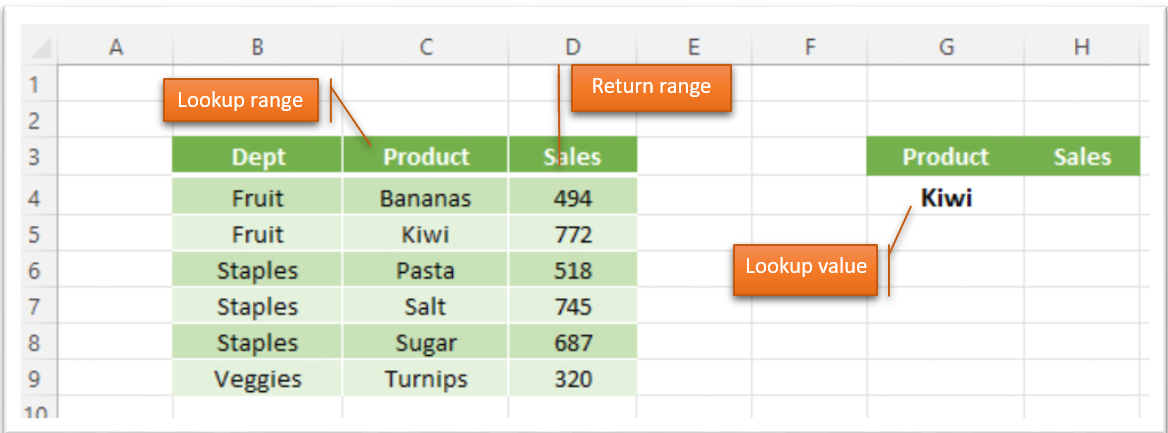
Suppose we have a table of data that contains information about different products in a grocery store. We want to use the XLOOKUP function to lookup the sales of a product based on its name.
In this case, the lookup range would be the Product list, the return column with the sales figures, and the search column would be the column that contains the names of the products. The lookup value would be the name of the product we want to look up.

Let’s search for the sales for Kiwi’s in this store. So, we want to find Kiwi in the product column and return the figure in the sales column.
- Lookup value – Kiwi
- Lookup array – the product column – C4:C9
- Return array – the sales column – D4:D9
Click on H4, enter =XLOOKUP(G4,C4:C9,D4:D9).

Using the XLOOKUP function, we can easily find out what the sales figures for Kiwis is.

Value If Not Found
When a value is not found in the XLOOKUP, the default value returned is #N/A. For example, there are no olives in the product list, so a search for olives should produce an error.
We could leave the error message as #N/A but users unfamiliar with Excel may think there’s an error with the worksheet. Creating a descriptive ‘if not found’ message informs the user that the value is not there, and that the product list needs to be updated.
In G4, type Olives. The formula returns #N/A.

To change the ‘if not found’ message, edit the formula. Enter your message text in speech marks. Click in H4 enter =XLOOKUP(G4,C4:C9,D4:D9,”Product not found”).

Match Mode
The match aspect of the XLOOKUP defaults to an exact match, which is useful for text. However, in some cases, an exact match is not required.
For example, in the table below, we have sales by person, and the commissions rate they earn are in the second table. Sales up to $98,000 earn 4%, while sales above 98,000 but less than 105,000 earns them 7% commission. As Joshua’s sales are over $98,000, he should earn a 7% commission.

In the sample data file, Match tab, in F4 enter =XLOOKUP(E4,H4:H10,I4:I10,,1). Notice the ‘if not found’ portion of the formula is empty. It is not needed in this case as we don’t expect the precise lookup values to be listed in this scenario.

Select column F, click the % icon on the Home.

Search Mode
The search mode lets you determine in what order to search the values in the lookup range, from first to last, last to first. For values in alphabetical order, you can choose to search A – Z or Z – A.
In this example, a local restaurant has a delivery service. A new order comes in for zone 3. There are two drivers work that area, both are available. We just need the first zone 3 driver on the list.

On the Delivery tab, in H4, enter =XLOOKUP(G4,E4:E11,C4:C11,”na”,0,1).

As we used the search mode 1, Excel searched from the first to last values, and the name Joe was returned.

Click in the cell or the formula bar, change the search mode (the last number in the formula) to 2, and Kwame’s name is displayed as Excel is now searching from last to first.
Returning multiple cells
By expanding the lookup array, we can return multiple cells. In the example below, we want to lookup both the Name and Department of an employee by using their ID number as the lookup value.

On the Employee tab, in G4 enter =XLOOKUP(F4,B4:B11,C4:D11,”na”,0,1).

Note that the return array in the formula includes both the Employee and Department columns.
Searching For Horizontal And Vertical Values
We can use XLOOKUP to return cell values at a horizontal and vertical intersection by creating a nested formula. In this example, we’re searching for the Security costs for Quarter 1.

The first part of the formula looks for the Security values, the second for the Q1 values. On the AP tab, click D3 enter =XLOOKUP(D2,B8:B12,XLOOKUP(C3,C7:F7,C8:F12)). This is an example of a nested xlookup formula.

Excel returns $33,796.00.
As the lookup values point to a cell, we can easily change the search without editing the formula. We can edit the search to view the Q2 figures. In C3, type Q2, the result updates to the Q2, Security figure of $31,812.00.

Using A Dropdown List In The Lookup Value Cell
To make it easier to change the lookup values, we can place the lookup value in a separate cell and use a dropdown list to change that value as needed. This option is especially useful for large datasets and eliminates the possibility of users making errors when entering search values.
On the List tab, click on C3. On the ribbon, click the Data tab, Data Tools, Data Validation.

The Data Validation dialog opens, in Allow select List.

In the Source field, click the arrow, we want to capture the list of periods, select C7:F7, press enter, OK.
An arrow appears in C3 with a list of the values from the range we selected.

Click the arrow in C3, select Q3, the formula returns $35,348.00.

We can repeat these steps to create a drop-down list for D2, using the Accounts Payable list.

Using XLOOKUP With The SUM Function
We can nest the SUM and XLOOKUP functions, allowing us to return multiple ranges of values and combine them for a total.

On the SUM tab, click E3, type =SUM(XLOOKUP(C3,B8:B12,C8:F12):XLOOKUP(D3,B8:B12,C8:F12)).
The formula uses the return range of all the data – C8:F12, thus Excel will return tthe total charge for Q1 through Q4 for each Accounts Payable category selected. Excel returns $499,000.00. This is the total cost for Insurance and payroll for all 4 quarters.

Change D3 to Security, the formula refreshes to the new total cost of $792,949.00.

Now you can use XLOOKUP like a pro!


Leave a Reply