How to Make an Ogive Chart in Excel: Step-by-Step Guide
It is a pity that the ogive chart is not a defined chart type in Excel. I sometimes use it and for this reason I have to do an ogive graph step by step. Below I will show you how to easily create an ogive chart in Excel.
Table of Contents
What is Ogive Chart
An ogive plot allows you to show the cumulative frequency of data values. Therefore, the cumulative frequency plot is always an ascending line that grows by leaps and bounds as you cross data boundaries.
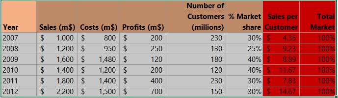
When inserting an Ogive (Cumulative Frequency) chart, the first thing you need is data like this:

As you can see in the picture above, the key step is to properly prepare the data table. When creating an ogive chart, you are faced with a difficult task.
The most difficult thing to do is to define the data ranges so that they do not disturb the frequency graph. When designing an ogive chart in Excel, it’s essential to try keeping your data intervals of the same size. Actually, it is from the point of view of the cumulative sum graph, so that they are of equal width.
In my example, I decided to create age brackets 15 years wide. In creating an ogive chart in Excel, it’s important to note that only the first compartment typically has a different width.It is allowed that the first and last bins have a different width. It is all the more acceptable when the data values in these ranges are small.
Write ages on an empty column (1), and write the last numbers in the ages (2).

Inserting a cumulative frequency
In column C, enter the upper ranges of the previously defined ranges. As I wrote earlier, it is 20 for me and each subsequent one is 15 more.
Remember that the task of the ogive chart is to show the sum of the accumulated data? In an empty column, write Cumulative Frequency and proceed to calculate the cumulative sum in column D below.
Click under the Cumulative Frequency, and type =B4, which is the value under Frequency in column B.

Click under the result from the previous result (1) and type =B5+B4.

Note: Follow this step on the rest, by typing =SUM(B6: B4 beside 50, =SUM(B7:B4) beside 65, =SUM(B8:B4) beside 80, and =SUM(B9:B4) beside 95.
Choose two cells under ages and cumulative frequency, right-click on them (1), and choose insert (2).

Choose to shift cells down (1), and press OK (2).

Put 0 under the cumulative frequency (1), and choose a number that rhymes with the ages under ages (2).
Highlight all of the rows in terms of both ages and cumulative frequency.

Inserting an ogive chart
Having calculated the cumulative frequency of your data, you can start creating a cumulative chart.
Ogive charts are usually scatter charts, but you can also choose to use a line chart. The important thing is that the plot should contain both a point and a line. I chose the scatter plot.
Select insert (1), scatter chart (2), and scatter chart with marker (3).

We have created an ogive chart that looks like this:

You can clearly see the value line that grows as the data ranges increase. At first glance, you can see that the greatest increase occurred between 35 and 50.


Leave a Reply