How to Create a Volatility Chart in Excel (Step-by-Step)
Standard deviation is a commonly used statistic in finance and economics to measure the volatility or risk of a security or portfolio. By plotting the standard deviation over time, you can create a volatility chart that shows how the volatility of a security or portfolio has changed over time. This type of chart is known as a standard deviation volatility chart.
Creating a standard deviation volatility chart in Excel is about understanding how a security’s volatility or price fluctuations have changed over a specific period of time.
Here is a step-by-step guide on how to make a standard deviation volatility chart in Microsoft Excel:
Data preparation
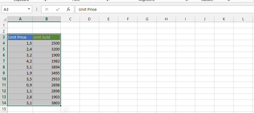
To create a standard deviation volatility chart, you will need to have a series of data points representing the returns of a security or portfolio. Make sure the data is organized chronologically, with the earliest data first and the latest data last.

Stdev formula
Calculate Standard Deviation in Excel on a daily basis. Click on the third cell from return and write, for example =STDEV(D6:D7), and then enter.
This will calculate the standard deviation of the data. Repeat this process for each period of time you want to analyze.

Click on the small square under the calculated result in the previous step twice.

Mark whole Changes column.

Note: This was chosen because it was based on how the stock performed at the end of the day.
Inserting volatility chart
Click on insert, lines, and line chart with marker.

Click on the chart (the design will show), and Click select data.

Click edit on the horizontal area.

Select all the dates, then press ok and ok.

Right-click on the Dates and choose Format Axis.

Change label position to low.

Click on the series (blue line).

Click on Add chart element, Error Bars, and Standard Deviation.

On the right side, scroll down to choose custom, and specify value.

Select the range in “Return”, for both Positive and negative error values, and press ok.

Our volatility chart looks like this:

Whether you are a business analyst, financial analyst, or data analyst, a standard deviation volatility chart can help you to quickly and easily analyze and communicate the volatility of your data.


Leave a Reply