Vlookup That Returns True or False
The VLOOKUP function in Excel can be used to return a value from a table based on a lookup value. However, sometimes you might want to return a simple True or False result based on whether or not a value exists in a table.
In this article, you learn how to create a vlookup formula which returns just true of false. You may need it to check if you have some data missing.
It is possible to create a vlookup formula which returns only boolean values – true or false.
To demonstrate how this can be done, let’s consider a simple example. Suppose you have a list of items and their prices in a table, and you want to determine if the price of a specific item is greater than a certain value. You can use the VLOOKUP function in combination with the IF function to accomplish this.
The syntax for the VLOOKUP function is as follows:
=VLOOKUP(lookup_value, table_array, col_index_num, [range_lookup])
Where:
- lookup_value: This is the value that you want to look up in the first column of the table.
- table_array: This is the range of cells that contains the data you want to search through.
- col_index_num: This is the column number within the table array that contains the value you want to return.
- [range_lookup]: This is an optional argument that specifies whether you want an exact match (FALSE) or an approximate match (TRUE) when searching for the lookup value.
The syntax for the IF function is as follows:
=IF(logical_test, [value_if_true], [value_if_false])
Where:
- logical_test: This is the condition that you want to test. It can be a comparison between two values, a test for a specific value, or a test for a specific condition.
- [value_if_true]: This is the value that is returned if the logical test is true.
- [value_if_false]: This is the value that is returned if the logical test is false.
To use the VLOOKUP function to return either “TRUE” or “FALSE”, you need to combine it with the IF function. The following formula demonstrates how this can be done:
ISNA formula
Let’s take a look at this example.
I created such a table.

I want to check if I have some data missing. For example I just type a customer’s name to check if I need to add it to my data table. In such example I need only true or false answer.
To check it I created such a formula: =ISNA(VLOOKUP($B$7,B2:B5,1,FALSE))
- ISNA – to not get an #N/A! error
- $B$7 – is an absolute reference to a value I know (customer’s name)
- B2:B5 – data range 1 – first column
- FALSE – because I need an exact match

IF and ISNA formula
Another examples would be to check if the guest is invited to the particular party.
I will use If function with ISNA as previously.
The formula is: =IF(ISNA(VLOOKUP(A4,$D$2:$D$5,1,FALSE)), “False”, “True”)
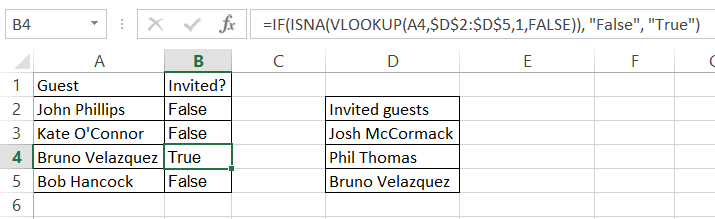
As you can see the formula recognized that one of guest is already invited to the party.
The formula used is preventing me before N/A! errors. Usage of IF function will return True of False as I needed.
Other conditions you may want to use this formula:
- to check if the client should get a discount
- to check if the student passsed get exam
- to check if the cleck should get a bonus
- to check if the item is present in the list
Of course this vlookup based formula can be used both for such basic data table and for advanced business intelligence dashboard.

Leave a Reply