How to Use Double Dash (–) in SUMPRODUCT Formula: Conditional Summation Guide in Excel
In any given condition, where we are looking for something specific within our data. Like how much we have made from one particular product, or how much we have made from one of our stores. Or any condition that we just want an answer to some part of the whole data.
The double dash (–) operator in the SUMPRODUCT formula provides an efficient solution for conditional data filtering and complex conditional summation tasks in Excel.
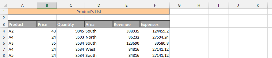
In this condition, we have sold our products in different places and have different products. But this time, we would like to know the net revenue from the South.
Data preparation
Suppose your dataset includes sales across various regions and products. You’re interested in the net revenue from the South region.

Inserting Sumproduct double dash formula
Click on an empty cell, and type in =SUMPRODUCT(–(D4:D8=”South”);E4:E8) – SUMPRODUCT(–(D4:D8=”South”);F4:F8).

Note: We’d subtract expenses from revenue for only the South. How you use the SUMPRODUCT with a double hyphen depends on what you would like the formula to obtain from the whole data set.
Let’s explore a few more scenarios where the double dash operator in a SUMPRODUCT formula can be handy for extracting specific information from your data in Excel:
Counting Occurrences
Suppose you have a dataset of customer feedback, and you want to count how many times a specific keyword appears in a column. You can use the double dash to convert the logical test into a numeric value, and then sum these values to count the occurrences.
=SUMPRODUCT(–(A2:A10=”Excellent”))
This formula will count the number of times “Excellent” appears in the range A2:A10.
Conditional Summation
If you have a dataset with various products and you want to find the total sales of a specific product, you can use the double dash operator to filter the relevant data.
=SUMPRODUCT(–(B2:B20=”Product A”), C2:C20)
This formula calculates the total sales for “Product A” from the dataset.
Weighted Average
Let’s say you have a dataset of test scores for students, and you want to calculate the weighted average for a specific subject. The double dash can help you apply weights to the scores based on the criteria.
=SUMPRODUCT(–(A2:A10=”Math”), B2:B10, C2:C10) / SUMPRODUCT(–(A2:A10=”Math”), B2:B10)
This formula calculates the weighted average of Math scores where B2:B10 represents the scores, and C2:C10 represents the weight for each student.
Filtering and Aggregating Data
You can use the double dash with other functions like SUMPRODUCT and AVERAGE to filter and aggregate data based on specific conditions. For instance, you can find the average revenue per order for a specific product category.
=AVERAGE(SUMPRODUCT(–(D2:D100=”Electronics”), E2:E100) / SUMPRODUCT(–(D2:D100=”Electronics”), F2:F100))
In this formula, you filter the data for the “Electronics” category, calculate the revenue per order, and then find the average.
Cost-Benefit Analysis
For financial analysis, you can use the double dash to compare costs and benefits. Suppose you have a dataset of investments and returns, and you want to find the net benefit for a specific investment type.
=SUMPRODUCT(–(A2:A20=”Stocks”), B2:B20) – SUMPRODUCT(–(A2:A20=”Stocks”), C2:C20)
This formula calculates the net benefit for “Stocks” by subtracting the total cost from the total return.
Now that you understand how to use the double dash operator in SUMPRODUCT formulas, you can apply this technique to streamline your data analysis in Excel.


Leave a Reply