The VLOOKUP function is a powerful tool in Excel that can be used to lookup values in a table. However, the VLOOKUP function can only lookup values in a single table at a time.

Consolidating data from multiple Excel files

To consolidate data from multiple Excel files, you can use the Consolidate function in Excel.

1. In the new Excel file, go to the Data tab and click the Consolidate button.
2. In the Consolidate dialog box, select the Function that you want to use to consolidate the data.
3. In the Reference field, select the ranges that you want to consolidate.

The data from the multiple Excel files will be consolidated into the new Excel file.

Using the VLOOKUP function to retrieve values from a consolidated Excel file

Once you have consolidated the data from all of the Excel files into a single Excel file, you can use the VLOOKUP function to lookup values in the consolidated Excel file.

To use the VLOOKUP function to lookup values in a consolidated Excel file.

For example, the following formula would lookup the value in cell A2 in the column B of the table_array:

=VLOOKUP(A2, table_array, 2)

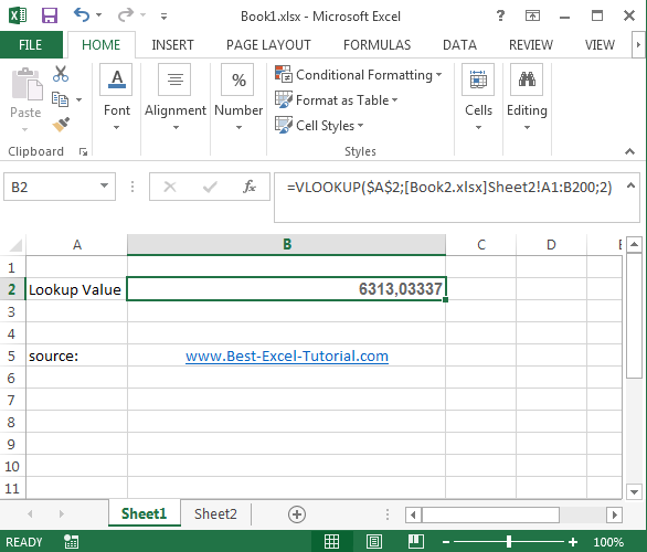
If the table_array is in another Excel file, you need to specify the name of the Excel file and the worksheet name in the table_array argument.

For example, the following formula would lookup the value in cell A2 in the column B of the table_array in the worksheet Sheet2 of the Excel file Example_Name.xls:

=VLOOKUP(A2, [Example_Name.xls]Sheet2!A1:B200, 2)

Using a combination of the VLOOKUP function and the INDIRECT function

We will show you how to use a combination of the VLOOKUP function and the INDIRECT function to retrieve values from multiple Excel files.

Steps:

1. Open the Excel file that contains the lookup values.
2. Create a new worksheet and name it “Criteria”.
3. In the Criteria worksheet, enter the names of the Excel files that contain the data you want to retrieve.
4. Select the Criteria worksheet and go to the Data tab.
5. Click the Advanced Filter button.
6. In the Advanced Filter dialog box, select the Criteria range option and specify the range of the Criteria worksheet.

This will create a new worksheet that contains all of the data from the Excel files that you specified in the Criteria worksheet.

Once you have created the new worksheet, you can use the VLOOKUP function to retrieve values from the data.

For example, the following formula will retrieve the value from cell A2 in the Sheet2 worksheet of the Book2.xlsx file:

=VLOOKUP($A$2,INDIRECT(“[Book2.xlsx]Sheet2!A1:B200”),2)

The INDIRECT function takes a text string as an argument and returns the value of the cell that is referenced by the text string. In this case, the text string is “[Book2.xlsx]Sheet2!A1:B200”, which references the range of cells in the Sheet2 worksheet of the Book2.xlsx file.

You can use this same technique to retrieve values from multiple Excel files. Simply enter the names of the Excel files in the Criteria worksheet and use the VLOOKUP function to retrieve values from the new worksheet that is created by the Advanced Filter.

See also  Vlookup for a range of values

Related posts:

How to Calculate Pv in Excel How To Use XLOOKUP Function In Excel How to Use VLOOKUP in Excel to Keep Formatting Consistent