In this lesson, you will learn about all the database functions in Excel.

Database functions are used to analyze data stored in a database. They have a few common features:

• Each function has three parameters: database, field and criteria. These parameters indicate the worksheet area used by the function.
• Except for the GETPIVOTDATA function, the other twelve functions start with the letter D.
• If you remove the letter D, you may notice that most of the database functions have already appeared in other types of functions in Excel. For example, if from DAVERAGE you remove D, this is well-known AVERAGE function.

General Syntax

Function_name (database, field, criteria)

• Database – range of cells, where your database is
• Field – name or numer of column where values are
• Criteria – your criteria should contain the name of the column and the name of some value from that column.

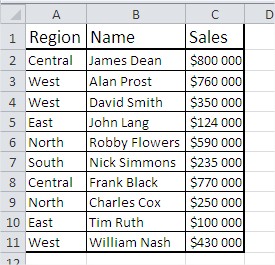
Let’s train that with examples. To use a database function in Excel, you’ll first need to set up your data in a format that Excel recognizes as a database. This typically involves organizing your data into columns and rows, and using headings for each column. This is an example database:

DAVERAGE

This function shows the average of values that meet your criteria.

The syntax for the DAVERAGE function is:

DAVERAGE(database, field, criteria)

where:

• “database” is the range of cells that make up your database, such as “A1:C10”.
• “field” is the column number that you want to average. For example, if you want to average values from column 2, you would enter “2”.
• “criteria” is the conditions that must be met for a cell to be included in the calculation. For example, you might use “A2:A10 = “Apples” to average only the values in column 2 that correspond to the “Apples” in column 1.

This is an example:

=DAVERAGE($A$1:$C$11;3;$A$1:$A$2) or =DAVERAGE($A$1:$C$11;”Sales”;$A$1:$A$2)

Note that the DAVERAGE function will only average cells that contain numbers. If a cell in the specified field contains text or an error value, that cell will be ignored in the calculation.

DCOUNT

This function shows the count of cells that meet your criteria.

The syntax for the DCOUNT function is:

DCOUNT(database, field, criteria)

where:

• “database” is the range of cells that make up your database, such as “A1:C10”.
• “field” is the column number that you want to count. For example, if you want to count values from column 2, you would enter “2”.
• “criteria” is the conditions that must be met for a cell to be included in the calculation. For example, you might use “A2:A10 = “Apples” to count only the values in column 2 that correspond to the “Apples” in column 1.

This is an example:

=DCOUNT($A$1:$C$11,3,$E$2:$E$3) or =DCOUNT($A$1:$C$11,”Sales”,$E$2:$E$3)

DCOUNTA

This function shows the number of noblank cells that meet your criteria. The DCOUNTA function works similarly to the DCOUNT function.

The syntax for the DCOUNTA function is:

DCOUNTA(database, field, criteria)

where:

• “database” is the range of cells that make up your database, such as “A1:C10”.
• “field” is the column number that you want to count. For example, if you want to count values from column 2, you would enter “2”.
• “criteria” is the conditions that must be met for a cell to be included in the calculation. For example, you might use “A2:A10 = “Apples” to count only the values in column 2 that correspond to the “Apples” in column 1.

This is an example:

=DCOUNTA($A$1:$C$11,3,$E$2:$E$3) or =DCOUNTA($A$1:$C$11,”Sales”,$E$2:$E$3)

Note that the DCOUNTA function will count all cells in the specified field, including cells that contain text, numbers, and error values.

DGET

This function shows a single value that meets your criteria.

The function has the following syntax:

DGET(database, field, criteria)

where:

• database: The range of cells that makes up the database. The first row of the range should contain the column labels.
• field: The column label that you want to retrieve the data from.
• criteria: A range of cells that contains the conditions you want to apply to the database. The first row of the criteria range should contain the column labels that correspond to the database.

This is an example:

=DGET($A$1:$C$11,3,A1:A2) or =DGET($A$1:$C$11,”Sales”,A1:A2)

If the criteria match multiple rows in the database, the DGET function will return only the first match it finds.

DMAX

This function shows the max value that meets your criteria.

The function has the following syntax:

DMAX(database, field, criteria)

where:

• database: The range of cells that makes up the database. The first row of the range should contain the column labels.
• field: The column label that you want to find the maximum value in.
• criteria: A range of cells that contains the conditions you want to apply to the database. The first row of the criteria range should contain the column labels that correspond to the database.

This is an example:

=DMAX($A$1:$C$11,3,$A$1:$A$2) or =DMAX($A$1:$C$11,”Sales”,$A$1:$A$2)

The DMAX function only returns the maximum value from a single column, not the entire row. If multiple rows in the database meet the criteria, the DMAX function will return the maximum value from the specified field for all matching rows.

DMIN

This function shows the min value that meets your criteria.

The function has the following syntax:

DMIN(database, field, criteria)

where:

• database: The range of cells that makes up the database. The first row of the range should contain the column labels.
• field: The column label that you want to find the minimum value in.
• criteria: A range of cells that contains the conditions you want to apply to the database. The first row of the criteria range should contain the column labels that correspond to the database.

This is an example:

=DMIN($A$1:$C$11,3,$A$1:$A$2) or =DMIN($A$1:$C$11,”Sales”,$A$1:$A$2)

The DMIN function only returns the minimum value from a single column, not the entire row. If multiple rows in the database meet the criteria, the DMIN function will return the minimum value from the specified field for all matching rows.

DPRODUCT

This function shows the multiplication of values that meet your criteria.

The function has the following syntax:

DPRODUCT(database, field, criteria)

where:

• database: The range of cells that makes up the database. The first row of the range should contain the column labels.
• field: The column label that you want to calculate the product of.
• criteria: A range of cells that contains the conditions you want to apply to the database. The first row of the criteria range should contain the column labels that correspond to the database.

This is an example:

=DPRODUCT($A$1:$C$11,3,$A$1:$A$2) or =DPRODUCT($A$1:$C$11,”Sales”,$A$1:$A$2)

If multiple rows in the database meet the criteria, the DPRODUCT function will return the product of the specified field for all matching rows. The DPRODUCT function only works with numeric values, and it will return an error if any of the cells in the specified field contain text or empty cells.

DSTDEV

This function estimates the standard deviation of values that meet your criteria.

The function has the following syntax:

DSTDEV(database, field, criteria)

where:

• database: The range of cells that makes up the database. The first row of the range should contain the column labels.
• field: The column label that you want to calculate the standard deviation of.
• criteria: A range of cells that contains the conditions you want to apply to the database. The first row of the criteria range should contain the column labels that correspond to the database.

This is an example:

=DSTDEV($A$1:$C$11,3,$A$1:$A$2) or =DSTDEV($A$1:$C$11,”Sales”,$A$1:$A$2)

If multiple rows in the database meet the criteria, the DSTDEV function will return the standard deviation of the specified field for all matching rows. The DSTDEV function only works with numeric values, and it will return an error if any of the cells in the specified field contain text or empty cells.

DSTDEVP

This function estimates standard deviation based on the whole population of values that meet your criteria.

It uses the following syntax:

DSTDEVP(database, field, criteria)

where:

• database: is the range of cells that makes up the list or database.
• field: is the column in the database that you want to base your calculations on. This argument should be a number that represents the column number.
• criteria: is an optional argument that allows you to specify certain conditions or criteria that the data in the field must meet in order to be included in the calculation.

This is an example:

=DSTDEVP($A$1:$C$11,3,$A$1:$A$2) or =DSTDEVP($A$1:$C$11,”Sales”,$A$1:$A$2)

DSUM

This function shows the sum of values that meet your criteria.

The syntax for the DSUM function is as follows:

DSUM(database, field, criteria)

where:

• database: is the range of cells that makes up the list or database.
• field: is the column in the database that you want to base your calculations on. This argument should be a number that represents the column number.
• criteria: is an optional argument that allows you to specify certain conditions or criteria that the data in the field must meet in order to be included in the calculation.

This is an example:

=DSUM($A$1:$C$11,3,$A$1:$A$2) or =DSUM($A$1:$C$11,”Sales”,$A$1:$A$2)

The DSUM function only works with lists or databases that have column headers. If your database does not have column headers, you should use a different function, such as SUMIF.

DVAR

This function estimates the variance of values that meet your criteria.

The syntax for the DVAR function is as follows:

DVAR(database, field, criteria)

where:

• database: is the range of cells that makes up the list or database.
• field: is the column in the database that you want to base your calculations on. This argument should be a number that represents the column number.
• criteria: is an optional argument that allows you to specify certain conditions or criteria that the data in the field must meet in order to be included in the calculation.

This is an example:

=DVAR($A$1:$C$11,3,$A$1:$A$2) or =DVAR($A$1:$C$11,”Sales”,$A$1:$A$2)

DVARP

This function estimates the variance of values that meet your criteria based on the entire population.

The syntax for the DVARP function is as follows:

DVARP(database, field, criteria)

where:

• database: is the range of cells that makes up the list or database.
• field: is the column in the database that you want to base your calculations on. This argument should be a number that represents the column number.
• criteria: is an optional argument that allows you to specify certain conditions or criteria that the data in the field must meet in order to be included in the calculation.

This is an example:

=DVARP($A$1:$C$11,3,$A$1:$A$2) or =DVARP($A$1:$C$11,”Sales”,$A$1:$A$2)