Vlookup for a range of values
Vlookup is a powerful function in Excel that can be used to search for a specific value in a range of cells and return a corresponding value from a different column in the same row. Doing vlookup for a range of values is also possible.
Here you have an example which shows you how to deal with vlookup for a range in Excel.
Vlookup formula with range of values
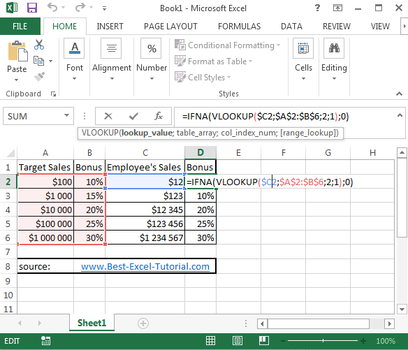
Your company set the new targets of sales. If employee reached the target, he will get a bonus. The higher target is the higher bonus. Let’s calculate the bonus using vlookup function.
Your formula looks like below:
=IFNA(VLOOKUP($C2,$A$2:$B$6,2,1),0)

How it works?
C2 – here is the lookup value
A2:B6 – this is a whole range of data (table_array)
2 – number of column in the range
1 – stands for approximate match
IFNA – this function checks if there is some bonus. If not it writes $0.
This is a simple example of how to perform a Vlookup for a range of values in Excel. You can modify the formula and the data as needed for your specific requirements.
Note: The above formula uses the Vlookup function with an approximate match, so it will return the closest value that is less than or equal to the search value. If you want an exact match, you can change the last argument in the Vlookup function from TRUE to FALSE.


Leave a Reply