How to Use Text to Columns in Excel?
In this lesson, you will learn how to separate the text written in one cell.
What does Text to Columns do?
Text to Columns is the option thanks to which Excel will separate text acoording to your needs and split it between columns. This option is used to separate text, usually copied from another source such as the Internet. Common delimiters include commas, spaces, tabs, slashes, and semi-colons. Excel allows you to select one or a combination of these delimiters based on how your data is structured. I prepared examples, where you’ll see how to use the Text to Columns.
Separate first and last names
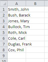
Here are names separated by a comma stored in one cell. You want to have them in two different columns. Text to Columns option is most often used to separate first name and last name from each. See how to do it.

How to separate from each other first and last name in Excel? It is very simple. Separating first and last name start with the selection of all cells.
Make sure that there is an empty space on the right hand side. If there is not, this is the point when you need to add additional columns on the right side. In other case you may lost the data which will be overwritten by splitted text.

Then go to the Excel ribbon. On the Data section there is an interesting option Text to Columns.
Note: To access this option, you can also use the keyboard shortcut ALT + A + E.

When you choose Text to Columns Wizard appears in text-to-column. In the first step, select the type of data format that best describes the data source. In this case it is a type Delimited, because the first and last name are separated by a comma.

In the second step, select the source text delimiters. In this case it is a comma. Immediately at the bottom of the dialog box you can see how Excel will allocate this text.

Skip the third step and leave everything as it is. Click Finish and verify results.

In this way Excel simply separated from each other names. Now they are in two columns instead of the one.
Fixed width
Let’s assume we have a list of ids imported from external tool.

We need to separate first 5 digits to the column B and the rest to the column C.
To separate fixed width text select that as in the picture above. Select Text to Columns button from the ribbon and pick Fixed Width option. Click Next.

In the next step drag a line to the desired position. In our case it is five digits from the left hand side. Click Next one more time.

The last step of the text conversion will require making two different decisions:
- You need to pick proper data format. I decided to leave it as General.
- The second decision is to select the Destination cell. This would be =$B$2 cell because I’d like to put data in columns B and C. You can also pick column A to replace previos data if you don’t need it any more. I decided to keep it to show you the change.

Here is how text has been converted to columns. You may see that first five digits are present in column B and the rest was moved to column C.

From the work experience I can share that fixed width conversion happen quite often. Usually I was using that during sales reports analysis when codes of products has been imported from external tools.
Text separated by spaces
The next example contains car names which are delimited by spaces.

We would like to separate a brand of the car from the model.
To separate a brand from its model similarly, select the data and click Text to Columns button from the ribbon above.
In the Convert Text to Columns Wizard pick Delimited option and Space as a delimiter.

Voila! This is how car brands and models has been separated in the spreadsheet.

Such kind of conversion is not being used so often. This is unusual to separate text by spaces by tools.
Your data should now be split into separate columns based on the delimiter you selected. If you ever need to undo the split, you can use the “Undo” button in the toolbar or press “Ctrl + Z” on your keyboard.


Leave a Reply