How to calculate ROIC?
In this lesson you can learn how to calculate ROIC in Excel.
What is ROIC?
ROIC stands for return on invested capital. Return of invested capital is one of the most basics measures in the business. ROIC is a profitability indicator which is used to measure the efficiency of the company, regardless of the structure of its assets or extraordinary factors. Return of invested capital should be higher than weighted average cost of capital.
ROIC is often used to compare with ROE. To understand ROIC, we must first understand ROE. ROE, then E refers to owner’s equity. It refers to the net interest rate which is calculated as dividing the net profit by the owner’s equity. ROE does have a downside. It ignores the leverage effect. Because many businesses such as finance and real estate have high net interest rates which is due to the high debt ratio.
IC refers to invested capital. Contrary to E, it treats a loan from a creditor to the company as a contribution and is included in the denominator. This is the biggest difference between ROIC and ROE.
ROIC calculations
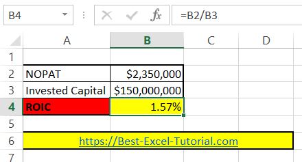
Let’s build the return on capital employed calculator in Excel. To calculate ROIC in Excel first you need some data. You need NOPAT and Invested Capital.
Copy and paste this roic formula in cell B4: =B2/B3
This formula will calculate the ROIC for data you place in cells B2 and C2 and is based on roic equation formula:
ROIC = NOPAT / Invested Capital
- Net Operating Profit After Taxes (NOPAT) is the company’s profit after accounting for all operating expenses and taxes, but before accounting for any financing or investment expenses.
- Invested Capital is the total amount of capital invested in the company, including equity and debt.
Remember to format ROIC as Percentage. Click B4 cell > click CTRL + 1 keyboard shortcut > click Percentage with 2 decimal places
Using XIRR function
Another method to calculate ROIC in Excel is to use the XIRR function. XIRR is an Excel function that calculates the internal rate of return for a series of cash flows that occur at irregular intervals. To calculate ROIC using XIRR, you need to create a series of cash flows that represents the invested capital and the returns generated by the company over a specific period.
Here’s a step-by-step guide to calculate ROIC using the XIRR function in Excel:
- Create a table with invested capital and returns: To use the XIRR function, you need to create a table that represents the invested capital and the returns generated by the company over a specific period. The table should have two columns, one for the dates of the cash flows and another for the amounts of the cash flows.
- Input the invested capital as a negative value: The first row in the table should represent the invested capital, which should be entered as a negative value. The date of the invested capital should be the date that the capital was invested in the company.
- Input the returns as positive values: The following rows in the table should represent the returns generated by the company, which should be entered as positive values. The dates of the returns should be the dates that the returns were generated.
- Create the XIRR formula: To create the XIRR formula in Excel, you need to use the following formula:
=XIRR(B2:Bn,A2:An)
Where B2:Bn represents the range of values for the cash flows and A2:An represents the range of dates for the cash flows.
- Calculate ROIC: Once you have created the XIRR formula, you can calculate the ROIC by hitting the “Enter” key. The result will be the ROIC for the company for the period being evaluated.
Using the XIRR function is another way to calculate ROIC in Excel. This method provides a more flexible way to represent the invested capital and returns generated by the company over a specific period, allowing you to account for changes in the invested capital and returns over time. As with the other method of calculating ROIC, it’s important to consider other factors such as revenue growth, profitability, and debt levels when making investment decisions.
Using SUM and IF functions
Next method to calculate ROIC in Excel is to use a combination of the SUM and IF functions. The SUM function can be used to calculate the total invested capital, while the IF function can be used to identify and isolate the NOPAT from the company’s profit and loss statement.
Here’s a step-by-step guide to calculate ROIC using the SUM and IF functions in Excel:
- Create a table with invested capital: To calculate the total invested capital, you need to create a table that lists the invested capital for the company, including equity and debt. The table should have two columns, one for the type of invested capital and another for the amount of invested capital.
- Use the SUM function to calculate the total invested capital: Once you have created the table with the invested capital, you can use the SUM function to calculate the total invested capital. The formula for the SUM function would look like this:
=SUM(B2:Bn)
Where B2:Bn represents the range of values for the invested capital.
- Create a table with the company’s profit and loss statement: To calculate the NOPAT, you need to create a table with the company’s profit and loss statement, including the revenue, operating expenses, and taxes. The table should have multiple columns, one for the type of item on the statement, and another for the amount.
- Use the IF function to identify and isolate the NOPAT: Once you have created the table with the company’s profit and loss statement, you can use the IF function to identify and isolate the NOPAT. The formula for the IF function would look like this:
=IF(C2=”Revenue”,D2,IF(C2=”Operating Expense”,-D2,IF(C2=”Taxes”,-D2,0)))
Where C2 represents the type of item on the statement and D2 represents the amount.
- Use the SUM function to calculate the NOPAT: Once you have used the IF function to identify and isolate the NOPAT, you can use the SUM function to calculate the NOPAT. The formula for the SUM function would look like this:
=SUM(E2:En)
Where E2:En represents the range of values for the NOPAT.
- Create the ROIC formula: To create the ROIC formula in Excel, you need to use the following formula:
= (NOPAT / Invested Capital) * 100
Where NOPAT represents the result from the SUM function for the NOPAT and Invested Capital represents the result from the SUM function for the invested capital.
- Calculate ROIC: Once you have created the ROIC formula, you can calculate the ROIC by hitting the “Enter” key. The result will be the ROIC for the company for the period being evaluated.
Using the SUM and IF functions is another way to calculate ROIC in Excel. This method provides a more detailed way to calculate the invested capital and NOPAT, allowing you to account for changes in the invested capital and NOPAT over time.
Using INDEX and MATCH functions
Another method to calculate ROIC in Excel is to use the INDEX and MATCH functions. The INDEX function can be used to find specific values in a table, while the MATCH function can be used to find the position of a value in a table.
Here’s a step-by-step guide to calculate ROIC using the INDEX and MATCH functions in Excel:
- Create a table with invested capital: To calculate the total invested capital, you need to create a table that lists the invested capital for the company, including equity and debt. The table should have two columns, one for the type of invested capital and another for the amount of invested capital.
- Use the INDEX and MATCH functions to find the invested capital: To find the invested capital, you can use the INDEX and MATCH functions. The formula for the INDEX and MATCH functions would look like this:
=INDEX(B2:Bn,MATCH(“Invested Capital”,A2:An,0))
Where B2:Bn represents the range of values for the invested capital, A2:An represents the range of values for the type of invested capital, and “Invested Capital” is the value you are looking for.
- Create a table with the company’s profit and loss statement: To calculate the NOPAT, you need to create a table with the company’s profit and loss statement, including the revenue, operating expenses, and taxes. The table should have multiple columns, one for the type of item on the statement, and another for the amount.
- Use the INDEX and MATCH functions to find the NOPAT: To find the NOPAT, you can use the INDEX and MATCH functions. The formula for the INDEX and MATCH functions would look like this:
=INDEX(D2:Dn,MATCH(“NOPAT”,C2:Cn,0))
Where D2:Dn represents the range of values for the NOPAT, C2:Cn represents the range of values for the type of item on the statement, and “NOPAT” is the value you are looking for.
- Create the ROIC formula: To create the ROIC formula in Excel, you need to use the following formula:
= (NOPAT / Invested Capital) * 100
Where NOPAT represents the result from the INDEX and MATCH functions for the NOPAT and Invested Capital represents the result from the INDEX and MATCH functions for the invested capital.
- Calculate ROIC: Once you have created the ROIC formula, you can calculate the ROIC by hitting the “Enter” key. The result will be the ROIC for the company for the period being evaluated.
Using the INDEX and MATCH functions is another way to calculate ROIC in Excel. This method provides a flexible way to calculate ROIC, allowing you to easily change the values in the tables without having to manually update the ROIC formula.
Leave a Reply