How to use Sum Function
In this lesson, you will learn how to use SUM function.
SUM function is probably the most used function of Excel. It is also really easy to use.
Sum function syntax
=SUM(number1,[number2],…)
Examples:
- =SUM(C2,C3,C5,C6)
- =SUM(B1:B4)
- =SUM(A1:C4)
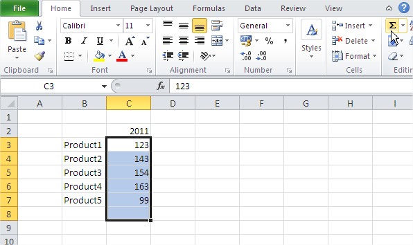
You can add in Excel also in several other ways. Excel will mark the safest area you want to sum up, along with the cell below or to the right where you want the sum. Just click on the icon bar or by press keyboard shortcut Alt + =.

Ten Examples of Using SUM Function
Open Excel and save your file as sum.xlsx.
The simplest example of SUM
To use the SUM function in its simplest form, click the cell E1 and enter the formula =SUM(50,100,25) and press the Enter key.

If you look at the formula bar, you can see the SUM function and in the E1 cell you can see the result 175 which is equal to the sum of 50, 100 and 25. Here, you have used comma (,) to separate the numbers inside the SUM function.
SUM of simple range
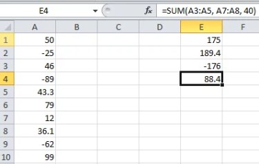
Enter a few numbers in the cells from A1 to A10. You can enter not only positive whole numbers, but also negative numbers or decimal numbers as well.

Suppose you want to calculate the sum of all the ten numbers. Click in the cell E2 and enter the formula =SUM(A1:A10).

The sum of the ten numbers is 189.4. Here, you have used colon (:) to select a number of consecutive cells, cells from A1 to A10.
SUM specific cells
Suppose you want to add only the negative numbers in the cells. Click in the cell E3 and enter the formula =SUM(A2,A4,A9).

SUM multiple ranges
Suppose you want to add numbers in cells A3, A4, A5, A7 and A8 and then add 40 to the result. Click the cell E4 and enter the formula =SUM(A3:A5, A7:A8, 40).

SUM with the LARGE function
Suppose you want to calculate the sum of the 3 largest numbers in the list. Click the cell E5 and enter the formula =SUM(LARGE(A1:A10,{1,2,3})).

If you analyze the values in cells A1 to A10, you could find that the three largest numbers are 99, 79 and 50. We have used the LARGE function inside the SUM function to get the three largest numbers in the list.
SUM with the SMALL function
Suppose you want to calculate the sum of the 4 smallest numbers in the cell. Click the cell E6 and enter the formula =SUM(SMALL(A1:A10,{1,2,3,4})).

If you analyze the values in cells A1 to A10, you could find that the four smallest numbers are -89, -62, -25 and 12. We have used the SMALL function inside the SUM function to get the four smallest numbers in the list.
SUM of other SUM
Suppose for each cell, you want to calculate the sum of the current cell and the next cell. For example, for A1 the result should be A1 + A2, for A2 the result should be A2 + A3 and so on.
Click the cell B1 and enter the formula =SUM(A1,A2). Copy the formula in B1 to cells B2 to B10.

Here you could find that the value in cell B10 is 99 because the value in A11 is 0 and hence =SUM(A10,A11) gives 99 itself.
SUM with logical values
Click the cell E7 and enter the formula =SUM(99,TRUE).

Here the result is 100 and the logical value TRUE is translated into number 1.
SUM of data in other sheet
Suppose you want to calculate sum of two numbers where the first number is in Sheet 1 and the second number is in Sheet 2. Enter a number; say 28, in the cell A1 of Sheet 2. Click cell E8 and enter the formula =SUM(A1,Sheet2!A1).

SUM numbers and strings
Click the cell E9 and enter the formula =SUM(20, 50, “5”).

Here the string value 5 is translated into a number.


Leave a Reply