How to Calculate Stochastic Indicator?
The Stochastic Indicator is a technical analysis tool used to identify overbought and oversold conditions in the market. It calculates the position of the current price relative to the high and low price over a specified number of periods.
In this Excel tutorial, you learn how to calculate stochastic oscillator in Excel.
Stochastic oscillator formula
Here is the Stochastic Indicator Formula:
%K=(C–H) / (H–L)×100
where
- C is the current closing price
- H is the highest high over the lookback period
- L is the lowest low over the lookback period
%K is plotted with another quantity, %D. %D is a simple moving average of %K over a defined smoothing period.
Stochastic oscillator calculation
Use this formula to calculate the Stochastic Oscillator.
If your
- Date is under column A
- Open is under column B
- High is under column C
- Low is under column D
- Close is under column E
- Then in column F
write this formula:
- =100*(E1-D1) / (C1-D1)
Start by organizing your data in a column format in Excel, with the date in one column and the close price in another.
Calculate the highest high and lowest low: Use the MAX and MIN functions in Excel to calculate the highest high and lowest low over the specified number of periods.
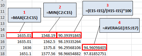
After applying these formulas, two lines oscillating on a vertical scale from 0 to 100 are created. The extreme values are determined by the levels of 80 and 20. They can be drawn on a graph in Excel, as I did below.
This will be your final result.
The sell signal occurs when the faster %K line crosses the slower %D line above the 80 level. The buy signal occurs when the %K line crosses the %D line from the bottom, i.e., below the 20 level.
Stochastic chart
Plot the Stochastic Indicator by using the %K and %D lines on a chart. You can use the chart wizard in Excel to create a line chart, and customize the chart to suit your needs.
To create a chart that visualizes the Stochastic Oscillator, follow these steps:
- Select the %K values (column F) and the corresponding dates (column A).
- Go to the “Insert” tab in Excel, and choose the chart type you prefer (e.g., Line Chart).
- Customize the chart to your needs, such as adding titles, labels, and other formatting options.
- Optionally, you can add horizontal lines at the 80 and 20 levels on the chart to help identify overbought and oversold conditions.
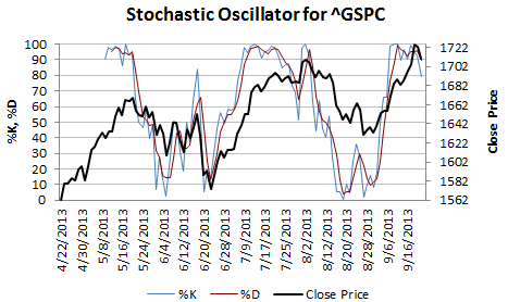
You can read these signals directly from the chart. The Stochastic Indicator provides insight into overbought and oversold conditions in the market. When the %K line crosses above the %D line, it is a bullish signal and suggests that the market is becoming overbought. When the %K line crosses below the %D line, it is a bearish signal and suggests that the market is becoming oversold.
This is how to calculate the Stochastic Oscillator in Excel.

Leave a Reply