How To Use Slicers In Excel
Learn how to use slicers in Excel to filter and analyze data more effectively. Excel slicers are interactive filtering tools that provide a powerful, user-friendly way to manage large datasets. This comprehensive guide teaches you how to use Excel slicers for data filtering, creating dynamic pivot table filters, and streamlining data analysis workflows. Master the slicers feature to enhance your data exploration capabilities and create more professional, interactive reports.
Table of Contents
What Is A Slicer? Understanding Excel’s Interactive Data Filtering Tool
So, what exactly is a slicer? In short, slicers are interactive filters that allow you to quickly and easily filter data in Excel. They’re incredibly easy to use. Simply click on the slicer element that you want to filter by and your data will be filtered accordingly.
Best of all, slicers can be used on any type of data, whether it’s numerical or categorical. You can create slicers from tables or Pivot Tables in Excel.
Benefits Of Using Slicers for Excel Data Filtering and Analysis
Several benefits come from using slicers in Excel.
First, they can save you a lot of time when filtering data. Rather than having to manually filter your data each time you want to look at a certain subset, you can simply use a slicer and have the work done for you.
Another benefit of using slicers is that they make it easy to share your data with others. Rather than sending someone an entire spreadsheet full of data, you can simply send them a file with the slicers already set up. This way, they can easily filter the data themselves without having to wade through everything.
How to Create Excel Slicers from Table Data
To create a slicer in Excel, you first need to have some data that you want to filter. Refer to the sample data in the How To Use Slicers In Excel.xlsx file. From there, you’ll be able to choose which element you want to use as your slicer.
Step-by-Step Guide: How to Create and Use Slicers in Excel
Open the How To Use Slicers In Excel.xlsx file, Table. Click any cell within the Excel table.
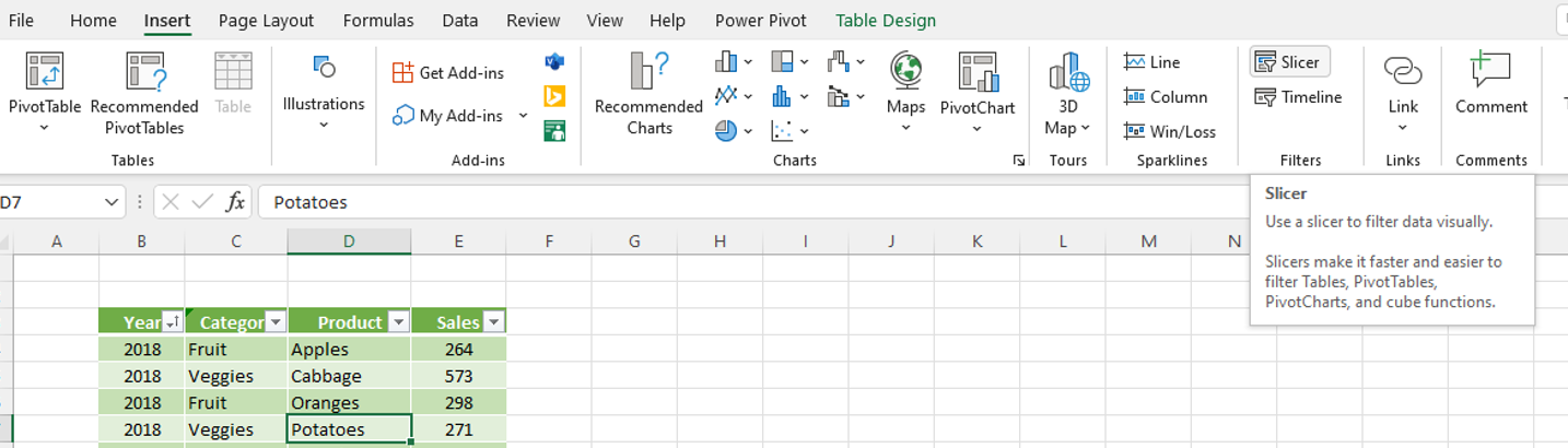
On the ribbon, click the Insert tab, Filters group, and click the Slicer button.

The Insert Slicers dialog opens. From here, you’ll be able to choose which element you want to use as your slicer. Select the Year, Product, and Sales elements, then click OK.

If the slicers are overlapping each other, use click and drag to separate them on the same row.

You can now use the slicers to filter the table data; Excel filters the data in place.
How to Select Individual Items Using Excel Slicers
In our sample data, we have the sales figures from a grocery store. We can use slicers to filter out individual items within each slicer.
- We want to see the apples sold in 2018:
- In the Year slicer, click 2018.
- In the Product slicer, click Apples.
- Excel filters the table to the relevant cells.
- Whenever you select a field within a slicer, the Clear Filter icon becomes active.

- Click the Clear Filter button in the Year and Product
- Excel displays all records in the table.
- Click the Sales figure 261. Excel displays the record for that sales figure only.
- Including the data field (sales in this example) in slicers is not very useful. Clicking on data fields will only return one record. A better practice is to create a slicer of all fields except the data field.
- On the Sales slicer click Clear Filter

How to Edit and Customize Excel Slicers
Once you’ve created your slicer, it’s important to remember that you can always go back and edit it if necessary. For example, if you want to change the fields you originally selected. This will allow you to make changes to the way that your slicer filters data.
- Let’s remove the Sales slicer:
- Click the Sales slicer, the border gets darker around it.
- Press the Delete key, Excel removes the slicer. Note you can also right-click on a slicer to access the Remove “Sales” option.
- Now we can create a slicer out of another field.
- Click any cell in the table.
- On the ribbon, click Insert, Slicer.
- The Insert Slicers dialog appears, click Category, then OK.
- Move the Category slicer in line with the others.
- We want to see the fruit sold in 2018:
- In the Year slicer, click 2018.
- In the Category slicer, click Fruit.
- Excel filters the table to the relevant cells.
- Notice that Excel displays all the products that fall under the category of fruit in the product slicers.
- Click the Clear Filter button on the Year and Category slicers.
Using Multi-Select for Advanced Excel Slicer Filtering
You can select more than one item within a slicer element.
Let’s filter the table to all the veggies sales in 2018 and 2021.
In the Year slicer, click the Multi-Select button; the button is yellow when active.

Click years 2018 and 2021. Note selected items appear as white within the elements. You can use the Multi-Select option on more than one slicer at the same time.
Click Veggies in the Category element.

Click the Multi-select option to deactivate it; the button is now white.
You can clear filters in a couple of ways:
- On each slicer click the Clear Filter button, this is useful if only one filter is active. ALT+C is the keyboard shortcut for this feature.
- Click the Clear button on the Data tab. To use this option, your cursor must first be in the table if you wish to clear filters on multiple slicers.
- How to Clear Excel Slicer Filters Efficiently
- On the ribbon go to the Data tab, Sort & Filter group, click Clear.

Slicers expand as you add data; the data refreshes and updates automatically.
Let’s add some data for 2022.
- Click in B28, type 2022, press tab. Notice the year appears in the Year slicer.
- In C28 press f, Fruit will appear.
- How Excel Slicers Refresh with New Data
- In E28 enter 424.
- In the Product element, click Jackfruit.
- The new entries appear in the slicers automatically.

The Slicer tab appears whenever your cursor is on a slicer. The options here allow you to change settings, formats, arrangement, and sizing.
Some useful features on this ribbon are:
- Under Slicer settings
- You can choose to hide records that have no data. This is useful if you have a table with blank cells.
- Buttons group
- How to Use the Excel Slicer Settings Ribbon

And two columns slicer:

Take the time to review the options on the Slicer ribbon to see what other features may be useful to you.
You can also create slicers on PivotTables; there are two ways to do this.
Adding PivotTable Slicers Using the Excel Ribbon Menu
Go to the Pivot tab of the worksheet. Click anywhere on the PivotTable. On the ribbon, click PivotTable Analyze.
How to Create and Use Slicers on Excel PivotTables

Click in the PivotTable, on the right side the PivotTable Fields pane appears.
Right-click on the Category element and click Add as slicer. The new slicer appears.
Adding Slicers to PivotTables via the PivotTable Fields Panel
Note, if there is more than one PivotTable in a worksheet, you can choose which one of them to include in your slicers by selecting Report Connections on the Slicers tab.

Overall, using slicers in Excel can be a huge help when it comes to data analysis. They’re easy to use and can save you a lot of time and effort in the long run.

Leave a Reply