If you want to learn how to calculate false position in Excel using the false position method for numerical root-finding, you are in the right place. We will explain what false position is, how it works, and demonstrate how to use the false position root-finding technique in Excel with a practical example.

How to calculate?

The example that we are using consists of five attributes. They are all placed well in a table.

We have two values that are already set, xl and xu. For the sake of this article, their values are 0 and 2.

We are first going to calculate f(xl) and f(xu).

We are going to use this formula:

=EXP(-x^2)-x-10

Replace all X’s with the coordinates of xl’s cell. In our case, the result we got was -9. We are going to do the same thing now with f(xu), and by doing that we got 42.5982.

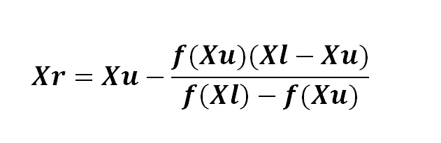
Now we have the intermediate value xr from the false position method calculation. We are going to calculate xr using the formula below, which is a key step in implementing the false position algorithm in Excel:

This may seem like a lot of brackets, but that’s because you have to replace all the X’s with the coordinates that match them.

The result we got is 0.34885. That’s how yours should’ve turned out if you followed the same example.

And the last thing that we have to calculate is f(xr). We are going to use the same formula that we used for calculating f(xl) and f(xu), and the result is -9.2194.

To fill up the other rows, are you going to start by creating a new xl and xu.

For a new xl use this formula:

=if(f(xl)*f(xr)<0,xl,xr)

For a new xu use this formula:

=if(f(xl)*f(xr)<0,xr,xu)

Copy and paste the rest and if everything works, you did it. You used the false position method.

Related posts:

How to get the cartesian product in Excel Earnings Per Share Calculator in Excel How to calculate logarithmic average in Excel