How to Show Year over Year Growth
In this Excel charting tutorial lesson, you will create a year-over-year report using a pivot table. You may need that for reports in Excel. Analysts will be especially happy because of that lesson.
Year over year data analysis
1. Select a cell in your data sheet.

2. Go to Insert ribbon’s tab and click on Pivot Table.

3. A dialog box will appear. Keep the default settings and click Ok.

4. A new blank worksheet will be created, containing a PivotTable Field List. Select your desired fields, that is Date and Revenue (for this example) that will appear in columns A and B.

5. Move the cell pointer to the first entry in column A.

6. Click on the Group Selection from the ribbon.

7. A Grouping dialog box will appear. Select years and months (or quarters whatever you want). Then click Ok.

8. The pivot table will illustrate the years and months stacked in an outline view. Drag the Quarters tile from the Row Labels to Column Labels from the bottom of the PivotTable Field List.

The new look of the report will be like this:

9. Go to the Design tab and from the Report Layout drop down list, click on Show in Tabular Form.

The gridlines will now appear.

10. From the Grand Totals drop down menu, select On For Columns Only to remove the Grand Total column that appears on the right side.

How to show year over year % growth?
The report will appear like this:

11. Then make a heading of % Change in 2013-14 in E4 and % Change in 2014-15 in F4.

12. In E5, type a formula =ABS(C5/B5-1) and in F5, type a formula =ABS(D5/BC5-1). Do not use the mouse or arrow keys to select any cell.

13. Now go to E5 and right click then select Format Cells.

14. A dialog box will appear. Click on Percentage and select the Decimal Places: 1 then click Ok.

15. Copy E5 down to all rows.

16. Repeat the steps 13-15 for F5.

17. Select the Sum of Revenues heading and go to the Options menu. Click in the Active Field box and write Revenues followed by a space.

18. Then click on the Field Headers so that they will not appear in the final report (if you want).

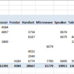
The final year-over-year report will be like this:

You now have a pivot table that shows the year over year growth in Excel. You can further customize the pivot table by adding a chart, changing the summary calculations, or filtering the data to show only specific years.
Leave a Reply