Adding average to the pivot table
In this Excel tutorial, you will learn how to add average column to the pivot table in Excel. This is a very useful and simple trick.
How to get average in pivot table?
In a pivot table, you can add the average of a set of values by following these steps:
1. Open the Excel sheet where your pivot table is created.

2. Place your cursor anywhere on the pivot table. A PivotTable Fields box will appear.

How to add an average in pivot table?
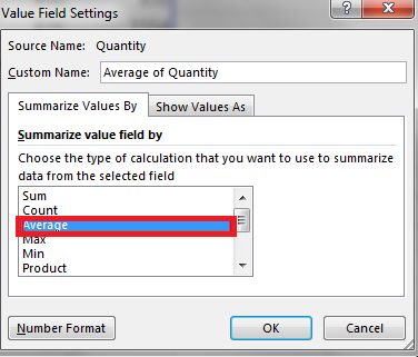
3. Right-click the sum of the quantity in the value box section and select value field setting. A dialog box will appear. Select Average in the Summarize value by tab and click ok.

4. Drag the quantity into the value box.

5. Refresh the pivot table. To update the pivot table with the average calculation, click on the “Refresh” button in the “Data” group on the “Analyze” tab in the Excel ribbon. The final result will be like this:

Your pivot table will now display the average of the values in the field that you selected. You can further customize the pivot table by adding more fields to the Rows and Columns areas, or by adding filters to focus on specific data.


Leave a Reply