Show Yes/No As the Values in a Pivot Table
Showing the yes/no value in the Pivot Table has multiple steps to it. See how to do that in Excel.
Yes no data preparation
To count the values of “yes no” in a PivotTable, you need the following data:

1. Click on an empty cell beside the value (1), and type =IF(B4>4500,”Yes”,”No”) (2). Finally, double click on the small square in the lower right corner of the result (3).

Inserting a pivot table
Unique yes no
2. Mark the data (1), click insert (2), and then click Pivot Table (3).

3. Click ok
4. Check a label, which in this case is the (name).

Note: Check the unique too.
5. Drag a name to the row, and then do the same with unique.

Note: The name and unique were dragged here.
The Pivot would look something like this:

Amount yes no
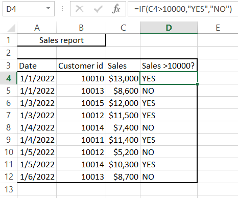
Examine the next case. You have received the sales report. This is a total sale, but you are only interested in trades over $ 10,000.
Add a column where you enter YES if sales are greater than $ 1000 and NO for the lower amount.
Use the if formula: =IF(C4>10000,”YES”,”NO”)
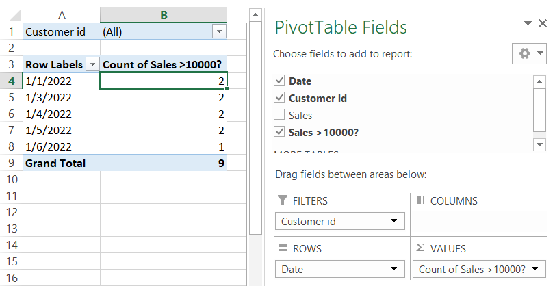
Create a pivot table. By adding an additional column, you now have the option to create a yes no sales report.
The pivot table below shows a report of the number of transactions over $ 10,000 per day.
Aggregate report yes no
Yes no data also allows us to aggregate.
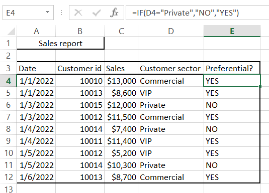
In this case, we have a sales report with 3 customer groups:
- private
- commercial
- vip
Private clients are not preferential for you.
You want to create a pivot table with sales values. You are only interested in preferential customers.
Create an additional column and, thanks to the if function, aggregate commercial and vip clients: =IF(D4=”Private”,”NO”,”YES”)
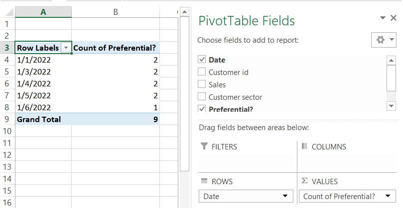
Thanks to the preferential column, you are able to create a pivot table showing how often your key customers make transactions.
An alternative method using Max
There is an alternative method to display Yes/No as the values in a Pivot Table. Here’s how you can do it:
- Create a Pivot Table by selecting the data range and clicking on the “PivotTable” button in the “Insert” tab.
- Drag the field that contains Yes/No values to the “Values” area in the “PivotTable Fields” pane.
- By default, Excel will count the occurrences of Yes and No values. Right-click on any cell in the “Values” area and select “Value Field Settings.”
- In the “Value Field Settings” dialog box, select “Max” instead of “Count” under the “Summarize value field by” section.
- Click on “OK” to close the dialog box and update the Pivot Table.
Now, you should see the Yes/No values displayed in the Pivot Table. The column headers will show “Max of” followed by the field name, and the cells will display “Yes” or “No” depending on the maximum value in each grouping. If there is at least one “Yes” value in a group, the cell will display “Yes.” If there are no “Yes” values, the cell will display “No.”
Leave a Reply