How to flip a chart in Excel
Why to create standard charts in Excel? Try something extraordinary. Let’s learn to create a chart from right to left. It means that that axis will flip on the right side of your chart. Just follow these steps.
Chart from Right to Left
Enter data into Excel sheet and select the data.

Go to insert and select any of the desired chart.

Right-click the vertical axis, then click format axis and go labels.

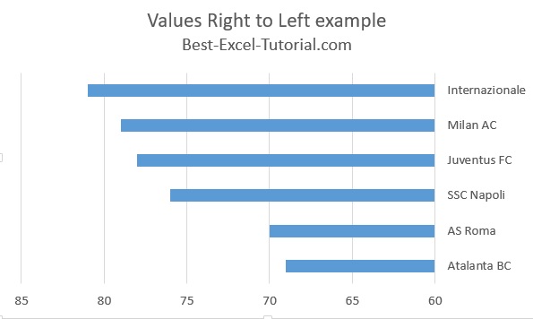
Now open the drop-down menu under labels and select high to move the vertical axis towards the left. Ready chart from right to left looks like that:

Here you can download a free Chart from right to left template.
Values in Reverse Order
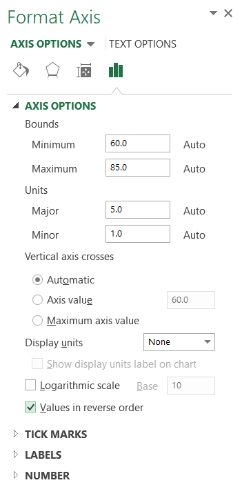
You can also set values in reverse order. Just right click your axis and choose Format Axis.
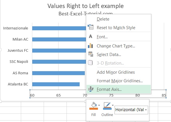
From the menu choose Values in Reverse order.
Now your bar chart is inserted from right to left.
This is how to flip a chart in Excel.
How to move X axis
If you are not satisfied with rotating your chart, then move the axis as well.
In Excel, you can move the axis so that it intersects the graph at the point that suits you.
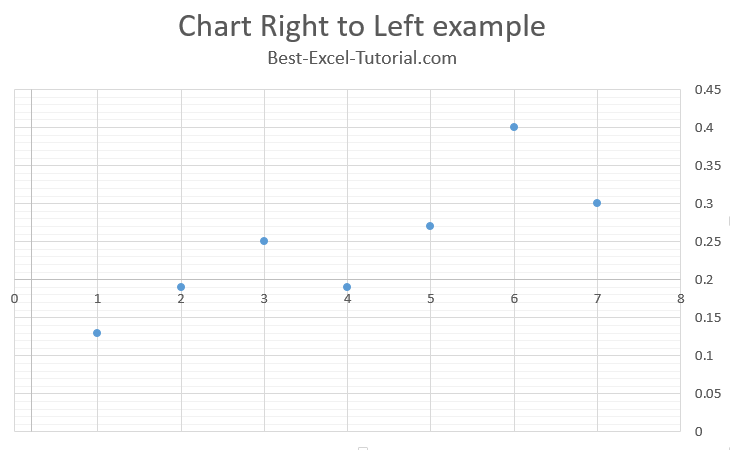
Now I will teach you how to move the x axis higher. I don’t want the x axis to be at the bottom of the plot. I will move the x axis higher in the chart.
I don’t want the x axis to cross the y axis at point 0. I want the x axis to intersect the y axis at 0.2.
It’s easy to move the x-axis up the chart. To change the position of the x-axis, left-click on it. In the Formax Axis menu, go to Axis Options. In the Vertical axis crosses field, click on Axis value and enter the value. I entered 0.2.
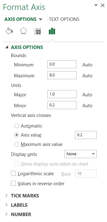
The x axis has moved and now intersects the y axis at 0.2.
I hope you enjoyed the trick.
Leave a Reply