How to Do Regression Analysis in Excel
Regression analysis is a powerful statistical tool used to analyze and model the relationships between variables. It allows us to understand how changes in independent variables affect the value of a dependent variable.
We will explore how to perform regression analysis in Microsoft Excel, specifically focusing on linear and multiple regression models.
Accessing Regression Analysis in Microsoft Excel
Enable the Analysis ToolPak:
- Click on File in the Excel ribbon.
- Select Excel Options.
- Click on Add-Ins in the left sidebar.
- In the Manage box at the bottom, choose Excel Add-ins and click Go.

Once you’ve enabled the Analysis ToolPak, you will have access to a range of data analysis tools, including regression.

Data Analysis button will appear on Data ribbon. Under Data Analysis feature Regression function can be found.

Regression Analysis in Excel
Prepare X & Y values in the following style.

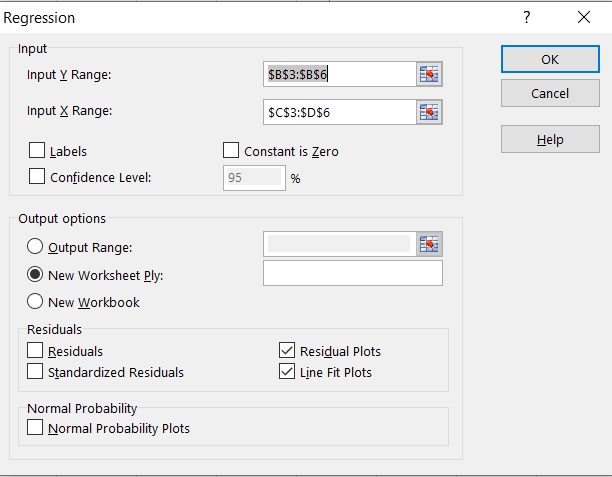
Open Data Analysis and choose the Regression.
Fill the dialog box with ranges of your data:
- Input Y Range option: Select dependent variables,
- Input X Range option: Select independent variables,
- Output options specify how you would like the results to be displayed,
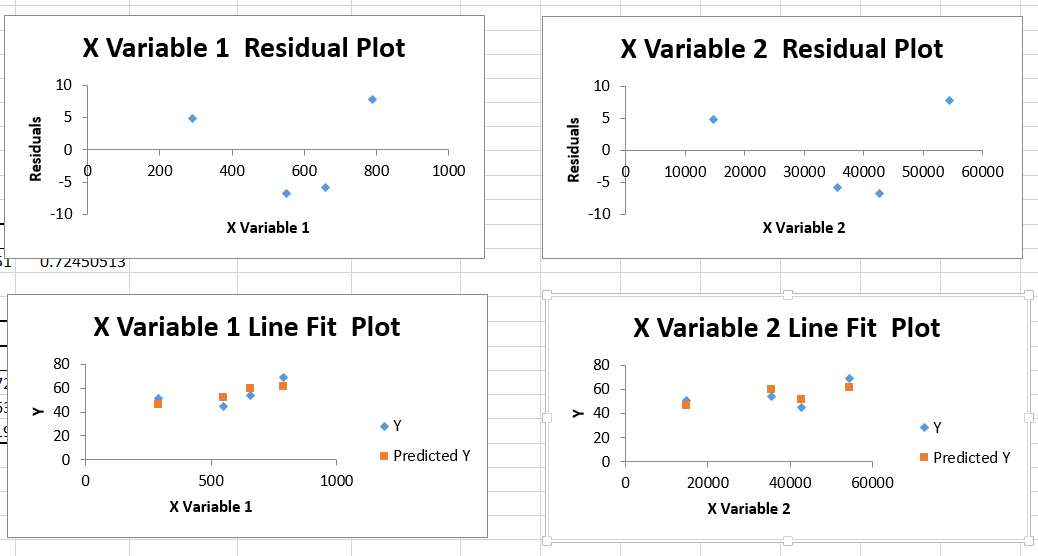
- Residuals contain options to draw the results as charts.

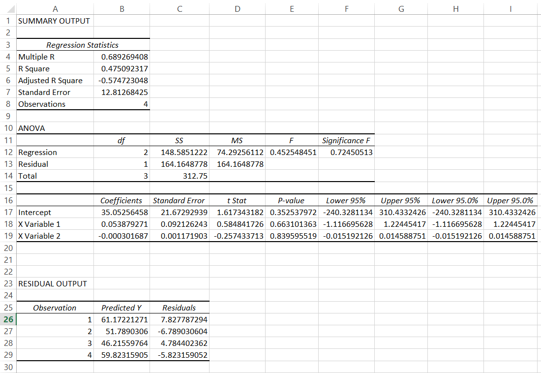
Following regression table will be created in new sheet as follows.

Linear Regression in Excel
The linear regression function answers the question: “What value will a given phenomenon (dependent variable) take, depending on the value of another phenomenon (explanatory variable)?” Due to the term “linear”, a method which has a way to remove the explained phenomenon and the variable explanation is precisely linear.
To run the linear regression prepare your data.

Select the cells for y-values, then the ones for x-values. Check the labels.

Insert a scatter chart.

Right-click on the chart and choose Select Data.

Write the Series Name, choose the cells for X-values, and for Y-values.

Click Ok.

Right-click on any of the markers and select Add Trendline.

Check the Display Equation on Chart and the R-square value on chart.

You should have done a linear regression that looks like this:

Multiple Regression in Excel
Multiple regression extends linear regression by considering the relationship between a dependent variable and multiple independent variables. Here’s how to perform multiple regression in Excel:
The first thing is having a data that could look something like this:
Choose the data you want to analyze on X values, and Y values. Select desired options, under the Residuals.
The multiple regression would look something like this:
Leave a Reply